Classify Images With A CNN

Image classification using a CNN & all of the dumb questions I had to Google in order to get here.

Built in `Python` using `Keras`

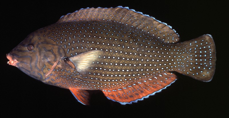
It’s been a long journey to get to where I am today, but I finally have some results to show for it! While I’ll refrain from describing the project in relation to Dr. Alfaro’s lab, I am excited to share my work in a more general sense. I want to talk about the problems that I couldn’t solve with a quick Google search, so if you’re looking for something comprehensive, mosey on. For this post, we will be classifying two classes of fish: Labridae and Gobiidae.


Labridae	Gobiidae

First of all, I’m going to assume that you know the basics of neural networks and CNNs. If not, let me guide you here. I felt that all of the concepts are clearly explained and easy to understand (If I can understand it, so can you!).

So here we go:

Part 1: Data preparation

I thought that this would be easy with a quick Google search, but I must have been using the wrong search phrase because I could not, for the life of me, figure out how to import my images easily. Most of the tutorials on CNNs used pre-packaged datasets that were built in with functions to resize, or that were already cropped and ready to go. Since I was dealing with images that were stored on my local machine, I had to figure out the steps necessary to clean my dataset. They turned out to be:

Walk through a directory and get the path of every image
Convert the image to pixel data
Resize the image to a standard length and width

I had used a few different functions to do the same task, but I settled with the walk function from the os library and the cv2 library from opencv.

from os import walk
import cv2

#Don't forget to change these paths!
lab = "~/Labridae"
gob = "~/Gobiidae"

fish_paths = []

for (dirpath, dirnames, filenames) in walk(lab):
    for i in range(len(filenames)):
        lab_img = dirpath + '/' + filenames[i]
        if "Store" not in lab_img:  
            fish_paths.append(lab_img)
    break

for (dirpath, dirnames, filenames) in walk(gob):
    for i in range(len(filenames)):
        gob_img = dirpath + '/' + filenames[i]
        if "Store" not in gob_img:
            fish_paths.append(gob_img)
    break

If you’re unfamiliar with the walk function, it returns three things:

root (str)
dirs (list)
files (list)

The root is the entire path to where the folder you passed into walk is stored. If I were to run walk('/Users/leann/Desktop/fish'), my root would be /Users/leann/Desktop. Dirs refers to any folders within the folder you passed in. So if I had 3 folders in '/Users/leann/Desktop/fish', the name of those three folders would be listed. Files is, as you guessed, all the files within '/Users/leann/Desktop/fish'.

We add root + '/' + files[i] to get the full path of the image.

It may seem a bit messy to add all of the image paths to one list, but I find it easier to keep track of one list, then pull data out of it to create testing sets. We will also create a separate list of labels, where the indices for the paths list and labels list match.

Next we need to standardize every image and create our classification labels.

x_train_ordered = []
y_train_ordered = []

for i in fish_paths:
    img = cv2.imread(i)
    # standardize size for prediction step
    img = cv2.resize(img, (150, 150))
    img = img/255.0
    #img = img.reshape((1,) + img.shape)
    x_train_ordered.append(img)

    if "Labridae" in i:
        y_train_ordered.append(0)
    else:
        y_train_ordered.append(1)

cv2.imread() returns 3-dimensional array of pixel values that range from [0-255] (RGB values). We divide each pixel by 255 to normalize the data and improve convergence. If you check the shape of the image, it should be (150,150,3), meaning that for each dimension in the 3D array, we have resized the image to 150 by 150 pixels. If we have a 4D array shape (3,150,150,3), the first 3 refers to 3 separate images that have the shape (150,150,3). We also start appending values to y_train_ordered; 0 referring to a Labridae fish, and 1 referring to a Gobiidae fish. In order to pass classification values into the CNN, we must use numerical values as labels.

NOTE: We are using the variable names x_train_ordered and y_train_ordered because the first half of the list is Labridae images, and the second half is Gobiidae. In the next step, we will shuffle the images to make sure that the order of images doesn’t affect the model’s decision making.

import random
to_shuffle = range(len(x_trained_ordered))
random.shuffle(to_shuffle)

x_train = []
y_train = []

for i in to_shuffle:
    x_train.append(x_train_ordered[i])
    y_train.append(y_train_ordered[i])

test_indices = sorted(random.sample(range(len(x_train)), 200),reverse=True)

x_test = []
y_test = []

for i in test_indices:
    x_test.append(x_train[i])
    y_test.append(y_train[i])

    del x_train[i]
    del y_train[i]

In this block, our goals are to:

Shuffle all of the images and labels in our x_train_ordered and y_train_ordered lists so that they still correspond with one another
Segment out a portion of our x_test and y_test lists to use as testing data

First we shuffle a list of integers that range from 0 to the number of images we have. We will use this shuffled list as a way to index from the original ordered images list. We now create our official x_train and y_train lists by appending values from x_train_ordered and y_train_ordered using our shuffled indices list. We maintain that the image matches up with the classification label by using the same index for both lists.

Next, we pull from our training data to create a testing set. Usually, testing data is about 10% of the training data, so I decided to pull 200 images. In order to randomly sample 200 images from the training set, we use random.sample to pick 200 indices at random from x_train and order them from greatest to least. This is an important step, because we need to delete the images that will be used in the testing set from the training set. If the indices are not in a descending order and we deleted an object at index 3 before an object at index 4, we would get and indexing error when trying to delete the object at index 4. This is because we deleted index 3, thus shifting index 4 to index 3’s position.

We’re almost there!

import numpy as np

x_train = np.asarray(x_train)
y_train = np.asarray(y_train)

x_test = np.asarray(x_test)
y_test = np.asarray(y_test)

This step is a little silly. It seems that the CNN will only work with numpy arrays, so I had to convert all of my lists. I’m sure we could have just started with arrays from the beginning, but I’m just so much more comfortable working with lists, so I went for those. Feel free to reformat!

And we’ve done it! We’ve finished the data prep, which admittedly took me more time than building the actual CNN. On to the next part.

Part 2: Actually building the network

Thanks to all of the predefined libraries on neural networks out there, this was actually the easiest part of the project.

from keras.models import Sequential
from keras.layers import Conv2D, MaxPooling2D
from keras.layers import Activation, Dropout, Flatten, Dense

# dimensions of our images.
img_width, img_height = 150, 150

model = Sequential()
model.add(Conv2D(32, (3, 3), input_shape=(150,150,3)))
model.add(Activation('relu'))
model.add(MaxPooling2D(pool_size=(2, 2)))

model.add(Conv2D(32, (3, 3)))
model.add(Activation('relu'))
model.add(MaxPooling2D(pool_size=(2, 2)))

model.add(Conv2D(64, (3, 3)))
model.add(Activation('relu'))
model.add(MaxPooling2D(pool_size=(2, 2)))

model.add(Flatten())
model.add(Dense(64))
model.add(Activation('relu'))
model.add(Dropout(0.5))
model.add(Dense(1))
model.add(Activation('sigmoid'))

model.compile(loss='mean_squared_error',
              optimizer='rmsprop',
              metrics=['accuracy'])

The first three blocks are really intuitive. You can see that we add three convolutions layers using relu activation and three pooling layers. These steps are explained and can be followed in the initial tutorial I linked. In the last block, we flatten the number of input nodes to just 1, our prediction output (Dense(1)). We then compile the network using the mean squared error function as the loss function. The loss function can be switched out for another, but the switch will not make a poor classifier any better.

model.fit(x_train, y_train, batch_size=32, epochs=7, validation_data = (x_test, y_test), verbose=1)

And finally we feed the data into the model we built! We provide thee important parameters, batch_size, epochs, and validation_data. Batch size refers to how many images of the total training set the model will take and process at a time. The smaller the batch size, the faster the computer can process it; however, the trade off is that it’s much harder to know when your loss function indicates convergence. The default batch size is 32, so sticking with it isn’t such a bad option. The number of epochs is the number of times the model will run through the entire training set. We use our testing data set as our validation set as unbiased data that will tell us how our model is performing. The validation dataset is not used to train the model, only to provide insight.

You’ll notice that verbose is also in there. It’s not imperative to fitting the data, but when set to 1, it gives us this nifty status as the model is being trained and helps us understand how our model is doing.

verbose

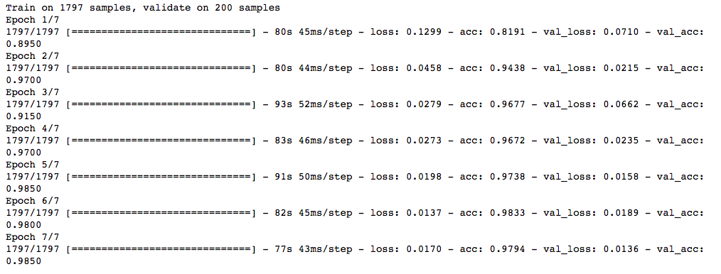
The four metrics the model outputs are loss, accuracy, validation loss, and validation accuracy. It’s intuitive that we want to minimize loss and have a higher accuracy, so we want to see loss and accuracy decreasing and increasing, respectively. We want to see the same pattern for validation loss and validation accuracy. If we see that validation loss keeps increasing while regular loss and accuracy decrease and increase, respectively, then we can assume that we are overfitting. The model is becoming too good at recognizing the training data, and cannot generalize outside of it.

Looking at these metrics is a good way to find the optimal number of epochs for your model. I started out with 10 epochs, and saw that validation loss started increasing instead of decreasing around 8 or 9 epochs, which is how I ended up at 7 epochs.

Part 3: Evaluating the model’s accuracy

Now that we have the trained model, we can see how effective it is at classifying the testing data.

from sklearn.metrics import confusion_matrix

predictions = model.predict(x_test).round()

confusion_matrix(y_test, np.squeeze(predictions, axis=1))

model.predict outputs a weighted value between 0 and 1, our classification labels. We use numpy.round to get integer values to compare the predicted values to the actual values. It also returns a multidimensional array, but in order to use sci-kit learn’s confusion_matrix function, it has to be 1-dimensional, so we use np.squeeze to get rid of the second dimension. By using a confusion matrix, we can quantify how many correct and incorrect classifications our model output.

confusion_matrix

113 images were correctly classified as Labridae, and 84 were correctly classified as Gobiidae. 2 images were incorrectly predicted as Labridae, and 1 image was incorrectly classified as Gobiidae. Overall, that’s 98.5% accuracy.

Next steps

We’ve successfully built a running model! Next steps would include analyzing the misclassifications and seeing how to fine tune the model to increase performance accuracy. This tutorial is extremely basic, but focuses on a lot of procedures and concepts that I had to spend a few hours trying to understand. I hope that you find it helpful, and if you have any questions, please feel free to email me. You can find the full code for this tutorial on my Github. Thanks for reading!